

This article is an excerpt from our “Mathematical Foundations for Reliability Block Diagrams” white paper.
Reliability Block Diagram (RBD) Analysis
One of the most useful tools in modeling a system’s reliability is the Reliability Block Diagram (RBD). It provides a way to graphically represent a system as a network of its base components and offers numerous calculations that demonstrate how these components contribute to overall system behavior. RBDs are highly versatile, applicable to simple cases, like series or parallel circuits, as well as more complex scenarios such as those involving repairable components or standby configurations.
To fully realize the benefits of using RBD for system analysis, it is helpful to understand the mathematical principles behind this powerful tool. This white paper investigates the mathematical processes that underpin RBD analysis. Topics include analyzing non-repairable and repairable systems, Monte Carlo simulation, important RBD metrics, standby redundancy, and more.
RBD Analysis for Repairable Systems
A system is repairable if at least one of its components is repairable. In addition to having a failure distribution, a repairable component also has a repair distribution. Once the component has failed, the repair distribution takes effect and influences the repair time. After the repair, the component again undergoes the failure distribution. In some scenarios, a component can carry over some prior wear after being repaired, causing it to resume partway through the failure distribution. For the purposes of this white paper, we assume that repairs are perfect. This means that components are restored to being as good as new, so the failure distribution takes effect as if it were starting from time t = 0 .
The behavior of switching back and forth between failure and repair distributions causes analytical calculations to become extremely difficult, if not impossible. The complexity also increases significantly with the number of repairable components. Fortunately, Monte Carlo simulation is a tool that works exceptionally well in these scenarios.
Monte Carlo Simulation
In the context of RBD analysis, the Monte Carlo method involves generating times from components’ distributions to simulate a possible run of the system. This process is repeated over many iterations, and then all the results are averaged to provide an estimate of the true results. As the number of iterations increases, the estimates will converge to the actual results due to the law of large numbers.
Random Time Generation
To better understand how this method works, it is important to know how a random time is generated from a probability distribution. This is done through a statistical process known as inverse transform sampling. First, we generate a random value uniformly distributed between 0 and 1, which is something a computer can do using a pseudorandom number generator. We interpret this number as the reliability of the distribution and work backwards in the reliability equation to solve for time. This time is our desired random value from the distribution. Note that a specific simulation can be reproduced using a random seed.
As an example, consider a Weibull distribution with shape parameter β = 1.5 and scale parameter η = 100. The reliability of this distribution is given by R(t) = e–(t/η)β . Rearranging this formula to solve for time gives t = η(-ln(R))(1/β) . Suppose our random number generated between 0 to 1 is 0.6, which we assign to the reliability. Solving for time, we have t = (100)(-ln(0.6))(1/1.5) ≈ 63.9021. This is the randomly generated time to fail or time to repair.
How a Single Iteration Works
Now we can demonstrate how a single iteration is completed for a repairable component. Assuming that the component is initially working, we first generate a random value from its failure distribution and use it as the failure time. Once the component has failed, we then draw a time to repair from the repair distribution and add it to the failure time to get the point in time when the component is repaired. After the repair, we add on the next generated time to fail, and the process continues as far in time as desired.
This gives us the time ranges when the component is working and when it is failed. Doing this for each component allows us to determine the periods of time when the system is in a failed state. Below is an example of how system states are derived from the component states.
Example Monte Carlo Simulation
Consider the following simple diagram. Suppose that we simulated an iteration up to 100 hours with these component state changes: Block fails at 30 hours and is repaired at 60 hours, block fails at 50 hours and is repaired at 80 hours, and block fails at 70 hours and is repaired at 90 hours.
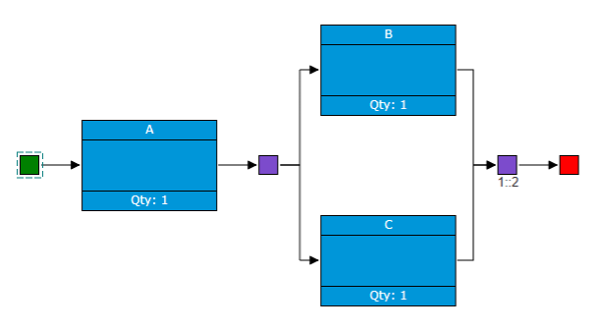
Path Sets
First, it can be helpful to look at all of the path sets of the diagram, which are all of the ways the system can succeed. In this case, a successful path can be traced from start to end through components A and B or though A and C, so at least one of these combinations must be working for the system to be active. In other words, the system is in a working state when the active component combinations are A and B, A and C, or A, B, and C. Next, we go through each component state change and see how they affect the overall system in the table below.
| Time in Hours | Active Components | System State |
| 30 | B and C | Failed |
| 50 | C | Failed |
| 60 | A and C | Working |
| 70 | A | Failed |
| 80 | A and B | Working |
| 90 | A, B, and C | Working |
This table shows the system fails at 30 hours, is repaired at 60 hours, fails at 70 hours, and is repaired at 80 hours. This information calculated over many iterations is all that is necessary to arrive at the key metrics for repairable systems.
Learn More
The “Mathematical Foundations for Reliability Block Diagrams” white paper covers the following extensive list topics:
- Non-repairable Systems
- Non-repairable System Metrics
- Reliability
- Failure Rate
- Computing System Metrics
- Series Configuration
- Parallel Configuration
- k-out-of-n Configuration
- Non-repairable System Example
- Non-repairable System Metrics
- Repairable Systems
- Monte Carlo Simulation
- Random Time Generation
- How a Single Iteration Works
- Example Monte Carlo Simulation
- Repairable System Metrics
- Availability
- Hazard Rate
- Reliability and Failure Rate
- Confidence Bounds
- Confidence Level
- Computing Availability with Confidence Bounds
- Example Repairable System Availability Calculation
- Monte Carlo Simulation
- Additional RBD Concepts
- Steady State Results
- MTTF
- Steady State Availability
- MTTR and MTBF
- Standby Redundancy
- Switching Mechanism
- Hot Standby
- Cold Standby
- Warm Standby
- Standby Configuration Calculations
- Effects of Standby Components on System Availability
- Steady State Results
Download the full white paper here. To learn more about Relyence RBD, feel free to contact us or schedule a personalized demonstration webinar. Or you are welcome to give us a free trial run today!