
For product designers and manufacturers, understanding how systems perform over time is essential for informed business decision-making. Once a product is in the field, its performance can be monitored through various data collection methods. However, turning that data into meaning insights, especially for evaluating overall reliability and forecasting future performance, can be a challenge. This is where Weibull Analysis becomes invaluable. By applying statistical techniques to analyze product life data, Weibull Analysis helps to assess reliability, identify trends, predict future outcomes, and ultimately make smarter, data-driven decisions.
What is Weibull Analysis?
Weibull Analysis is a statistical methodology used to analyze life data, evaluate product performance, and predict trends by identifying the probability distribution that best fits the data set. While the Weibull distribution is commonly used—giving the method its name—other distributions such as Normal, Lognormal, and Exponential may also be appropriate. The Weibull distribution is especially valued for its versatility, ability to work with small data sets, and effectiveness in modeling a wide range of life behaviors. As a result, Weibull Analysis is applied across various industries to assess product life data.
The core of Weibull Analysis involves collecting a sample of product failure data over a specific time period and applying statistical techniques to fit this data to a probability distribution. Once the best-fitting distribution is identified, you can evaluate key performance metrics. For example, you can estimate the mean life of a system, predict failure rates, calculate the probability of system survival over a given time interval, and assess appropriate warranty periods.

What is Life Data Analysis?
Life Data Analysis is a method of analyzing a sample set of failure data to predict how a product will operate over its lifetime. This analysis is done by fitting the data to a statistical distribution and using that distribution to determine trends. The term Life Data Analysis is used because it relies on real-world, field-based data that is analyzed to make forecasts about a product’s life. Though Life Data Analysis is the broader term, Weibull Analysis is often used interchangeably with Life Data Analysis as one of the most applicable distributions used in Life Data Analysis is the Weibull distribution.
The analysis methods and techniques are the same for both. The term Weibull Analysis has become so prominent due to the versatility of the Weibull distribution—it can be used to characterize a wide range of data trends that other statistical distributions cannot, including decreasing, constant, and increasing failure rates. In addition, the Weibull distribution can effectively be used to approximate other distributions, making it a powerful and flexible tool for reliability analysis.
Why perform Weibull Analysis?
Weibull Analysis enables you to leverage life data to drive product improvements throughout its lifecycle. By capturing product failure data and applying the statistical principles used in Weibull Analysis, you can work towards product improvements on a variety of fronts: help uncover the root causes of failures, determine the expected life of a product, predict product failure rate, optimize warranty periods, and more. Overall, there are four main advantages of Weibull Analysis:
- Prediction
- Analysis
- Planning
- Decision Making
Prediction
Using your life data, Weibull Analysis can help predict potential future failure characteristics. By identifying when failures are likely to occur, it enables you to estimate product lifespan and anticipate potential issues. By understanding the failure profile of your product, you can project future failure returns or repair needs. It can aid in forecasting warranty costs and helps quantify risk. These insights can help you optimize maintenance schedules, inspection intervals, and replacement times.
Analysis
Weibull Analysis results provide valuable insight into product performance. For example, by examining the shape of the best-fitting distribution, you can determine the nature of the failures occurring. If the best fit curve follows the Weibull distribution, the shape parameter, also known as the beta value, indicates failure type:
- A value less than 1 is indicative of early life failures
- A value equal to 1 indicates that failures are occurring randomly during the constant failure rate portion of the lifecycle
- A value greater than 1 indicates wear-out failures
This information helps you pinpoint which phase of the product lifecycle is most problematic and may require attention.
Weibull Analysis enables you to quantify important metrics such as MTTF (Mean Time to Failure), reliability at a particular time point, and life expectancy. By using these metrics in conjunction with Weibull plots like Failure Rate vs Time, you can objectively evaluate product performance. Additionally, analyzing Weibull results can help identify weak points in product design or in the manufacturing process, enabling you to target areas for improvements.
Planning
Using the information obtained from Weibull Analysis, you can effectively plan and organize maintenance strategies by scheduling maintenance before failures occur. This helps reduce unplanned downtime, minimize emergency repairs, and optimize spare parts inventories.
Decision Making
The results of Weibull Analysis can help to provide a metrics-based approach for product design improvements. By reviewing failure profiles and evaluating root causes, quality initiatives can target the most critical areas. Overall, Weibull results help drive informed decisions to improve safety, reliability, and quality.

How do I perform Weibull Analysis?
Performing Weibull Analysis involves collecting failure data and applying statistical methods to fit that data to a probability distribution. Once a best-fit distribution is identified, key reliability metrics and trends can be derived to support decision-making throughout the product lifecycle. The step-by-step process to perform Weibull Analysis includes:
- Collect failure data
- Analyze the data
- Interpret the results
- Make decisions
Step 1: Collect failure data
The first step in Weibull Analysis is to collect the data on the system you want to analyze. There are various ways to obtain this information. This data is often recorded in a corrective action system, such as FRACAS (Failure Reporting, Analysis, and Corrective Action System) that keep track of failure reports and other information relevant to the failure, such as repair times and recommended corrective actions. The advantage of using the data in a corrective action tracking system is that it represents real-world data. In other cases, you may have test data, such as run-to-failure results. Essentially, you want to collect a basic set of data that lists at the times at which failures occurred.
Additional information, such as the number of failures at a specific time, is also helpful and valuable to include. If the specific times at which failures occur are not known, time intervals may be used instead. You can also include items that did not fail during the testing interval. These are considered suspensions and help provide a more complete life data profile.
Step 2: Analyze the data
After data collection, the second step is to determine the mathematical distribution that most closely aligns to the data. This is typically done using a software tool designed for Weibull Analysis. These tools offer a best fit analysis feature which evaluates the various distribution types to assess which one best fits the sample data.
This resulting best fit may be the Weibull distribution, or a different distribution commonly supported in Weibull Analysis such as the Normal, Lognormal, or Exponential distribution.

Step 3: Interpret the results
Once the data has been fit to a distribution, the next step is to review and interpret the results. A Weibull Analysis software tool is again valuable at this stage of the process. Weibull software tools provide a set of helpful plots which make it easy to view graphs such as Reliability vs Time. Also, an analytics calculator provides the ability to compute a number of informative statistics based on the data analysis results.
Weibull Plots
A key element of Weibull Analyses are Weibull plots which provide the graphical representation of failure data along with the distribution curve. Weibull plots enable you to visualize your life data with the fitted distribution line for full understanding of trends and future performance.
Some common plot types that are used in Weibull Analysis include Probability, Reliability vs Time, Unreliability vs Time, Failure Rate vs Time, and PDF (Probability Density Function) plots.
Step 4: Make decisions
The final step, and the core objective, of performing Weibull Analysis is to use the results to make informed decisions that support your goals and drive success. There are several ways to apply the insights gained from Weibull Analysis. By examining trends in your Weibull plots, you can predict future product performance. If the projections align with your performance targets, you can have confidence in your product or system design. If the results fall short, you will need to identify and implement corrective actions—such as optimizing the design, enhancing maintenance strategies, or improving quality control processes.
Weibull results can also be used to anticipate spare parts demand, leading to more efficient inventory management. Additionally, they play a valuable role in managing and optimizing warranty programs, ensuring better cost control and customer satisfaction.

Example Weibull Analysis
To illustrate a practical use case for Weibull Analysis, we will look at a sample data set of 500 electric motors that were manufactured and shipped at the same time. Using data collected through a FRACAS, we have recorded failure reports from the first six months of use. Using that data, we want to project how the motors will perform over the next two years.
This analysis allows us to determine if our motors are performing as expected and enables proactive planning for future replacements. Specifically, we want to see if our motors are likely to maintain a high level of reliability, targeting at least 0.90 reliability, for the next two years, and also evaluate performance beyond that point.
For our example, we will use Relyence Weibull software.
Step 1: Collect failure data
As mentioned, we obtained failure times based on reports from an internal FRACAS. Over six months, ten failures were reported. One of the benefits of Weibull Analysis is that it provides meaningful results with a small sample set, so this data set will be sufficient to start our analysis. We will use the equivalent number of hours for the dates of the reported failures as the failure Time value for our Weibull data set. In addition, we know that 490 of the motors have not failed in this timeframe, so we will include that in our data as well as suspensions.
Here is our sample data set:
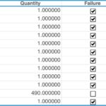
Data set for our electric motors. (Note that time is in hours.)
Step 2: Analyze the data
Now we need to find which probability distribution is the best fit for the data. Relyence Weibull has a Best Fit Distribution feature, so we will use that to determine the best fit. The Best Fit Distribution results show us the Residual for each distribution, which indicates the quality of the fit. The higher the value, the better the fit. The results are sorted in order of best fit.
Using a Best Fit analysis, we can see that the 3 Parameter Weibull distribution is the best choice for our data set with a residual value of 0.9888 indicating an excellent match for our data set.

Step 3: Interpret the results
Now that the distribution analysis is complete, it is time to review and interpret the results.
Weibull Plots
Weibull Plots provide a visual view of the results and can be easier to interpret than raw distribution parameters. One plot that is helpful is the Reliability vs Time plot, which gives us a view of the reliability of our motors over a time period.

Reliability vs Time Plot scaled to show Reliability at Two Years (17520 hours).
From the Reliability vs Time graph, we can see that reliability decreases over time, which makes sense. From the plot, we can see that our estimated reliability at two years (17,520 hours) falls between 0.95 and 0.96. This plot also includes two red lines which display the 90% lower and upper confidence bounds for our data. The confidence bounds are added as an indicator of the upper and lower values of reliability for our motors. This means that we can be 90% confident that the actual reliability at that point in time will lie between these bounds.
Weibull Analytics
We can also delve a bit deeper into the metrics to get more specific information. For example, we’d like to know the reliability values of our motors over a two year time period along with the upper and lower bounds. Relyence Weibull includes an Analytics Calculator tool to obtain these metrics.

Use the Analytics Calculator for more specific metric analysis.
The estimated Reliability (noted in the Value field) is 0.958444. The analysis also provides confidence interval, showing we can be 90% confident that our reliability at two years is between 0.94166 and 0.970475.
Step 4: Make decisions
In this case, our two-year estimated reliability meets our 0.90 reliability goal. If the reliability had fallen short of this objective, we could use this evidence to promote the need for product improvement. Using more analysis techniques available in Relyence Weibull, we can work to determine if failures tend to be early life versus wear-out failures, evaluate an appropriate warranty time, and more. In this way, we can work with our team to develop an action plan to improve the product’s design, manufacturing, maintenance, or a combination of all facets. This is why Weibull Analysis can be helpful throughout the entire organization.
Now, we want to take a look at our reliability estimate at ten years. Again, we engage the Analytics Calculator.

The Analytics Calculator provides more insight into failure trends.
Our reliability decreased some, as expected, but is still within our target range. Note that our confidence bounds have expanded, so our reliability has a range of 0.881486 to 0.940885. Because of this variability and because we want to have a better indication that our reliability is remaining above 0.90 at ten years, we want to reassess our reliability over the next six months. We will continue to track failures using FRACAS and then repeat our Weibull Analysis at that time. With additional life data, our estimates will be more accurate, allowing us to narrow our range of projected reliability values.
For another example of performing Weibull Analysis, check out our Introduction to Weibull Analysis blog post.
Weibull Analysis and Your Relyence Reliability & Quality Toolset
Relyence Weibull integrates seamlessly with other tools in your Relyence reliability and quality toolset, enhancing your ability to analyze and act on life data.
Weibull Analysis can be used in conjunction Reliability Block Diagram (RBD) analysis. If you have life data for a particular component of your RBD, you can enter that information into Relyence Weibull to determine the best fit distribution. Those results can then be used in Relyence RBD to define the component’s failure profile, enabling more accurate system-level analysis.
Weibull Analysis and Reliability Prediction analysis share a key feature: they are both predictive tools in reliability engineering. While Weibull Analysis uses life data, Reliability Prediction uses statistical analysis from historical data and device characteristics to estimate failure rates. Used together, they provide more complete and accurate predictions. For example, if you have a new system in development that includes some subsystems that are already in use in an older design or in a similar product already deployed, you can use field data from those subsystems in Weibull Analysis to refine your Reliability Prediction model in Relyence. In this case, you can augment your Relyence Reliability Prediction analysis by modeling those fielded components using Weibull techniques based on your collected life data.
As shown in our example above, FRACAS provides an excellent source for product life data. This life data can be used as a basis for Weibull Analysis. Relyence FRACAS includes a unique feature to automatically generate a Weibull Data Set from collected data. In this case, you can leverage your FRACAS data to create a unique forecasting system in addition to its effectiveness as a process management tool.

Relyence Weibull
Relyence Weibull provides an efficient platform for performing life data analysis. It includes a range of features to make Weibull Analysis quick and effective—such as a Best Fit analyzer, easy-to-read plots, an Analytics Calculator, and more.
Take Relyence Weibull for a free test drive today, contact us to discuss your needs, or find a time for a personalized tour with one of our knowledgeable team members.