Reliability Prediction is a widely used technique to analyze an electro-mechanical system in order to determine its expected failure rate or MTBF (Mean Time Between Failures). Estimated failure rate and MTBF values from Reliability Prediction analyses are effective and useful indicators of product reliability and quality. Therefore, Reliability Predictions are a useful tool to help you meet your product performance goals.
Reliability Prediction’s historical roots are in the military and defense sector, but over the years the technique has been adapted and broadened for use in a wide range of industries. Essentially, the advantages afforded by Reliability Prediction analysis make it an important part of managing and maintaining reliability and quality objectives.
What is Reliability Prediction?
Reliability Prediction is one of the most common techniques used by engineers to evaluate product and system reliability. As its name implies, Reliability Prediction is a predictive methodology that enables you to estimate, or predict, your system’s failure rate. Though an estimation methodology, the underlying analytical analysis used in Reliability Prediction has a strong statistical foundation. This means that the computed failure rate and MTBF values provide an accurate indicator of your product’s expected performance.

How Does Reliability Prediction Analysis Work?
To perform Reliability Prediction analysis, Reliability Prediction standards are employed. Reliability Prediction standards define an extensive set of equations used to model the failure rates of the various part types. Using the equations allows the overall product failure rate to be computed. Some of the most commonly used and widely accepted Reliability Prediction standards include MIL-HDBK-217, Telcordia, 217Plus, IEC 61709, SN 29500, NSWC Mechanical, and ANSI/VITA. The equations delineated in the standards were built by analyzing a huge amount of field data over a long period of time. Statistical analysis was then used to develop equations that best modeled the failure characteristics of the accumulated data.
The equations in the Reliability Prediction standards take into account the factors that affect the reliability of devices – such as operating stresses, temperature, environment, and procurement quality level. The factors used vary depending on the type of component being analyzed. When performing a Reliability Prediction analysis, you make a list of all the components of your system, find the appropriate equation in the standard for each component, evaluate the factors needed to compute the failure rate of each component, and then perform the failure rate calculation for the system. The cumulative sum of all the component failure rates is the total failure rate of your system.
The Reliability Prediction Standards
The failure rate equations used vary both across the standards and within each based on the various device types that are modeled. Depending upon your industry’s needs, one standard may be the most applicable. Or, in some cases, the standard to employ may be driven by compliance requirements. You may also choose to use a combination of standards. For example, a useful pairing is MIL-HDBK-217 and NSWC Mechanical. This combination provides a broad range of device models to select from with MIL-HDBK-217’s coverage of electronic devices and NSWC’s focus on mechanical components.

In addition to the equations used to evaluate the failure rate of individual devices, some of the standards provide supplementary techniques to improve your assessments. For example, the Telcordia standard allows you to incorporate laboratory test data and/or field failure data to refine predicted failure rates based on “real world” captured information. Telcordia also offers the ability to compute the confidence level of failure rate values and determine early life factors.
Each standard is very comprehensive, and we will not delve in-depth into all the details of each individual standard in this article. However, our in-depth guide on reliability prediction standards does just that! It provides detailed information on the differences between the various methodologies and offers advice to help you determine which is most applicable for your use.
What is the Bathtub Curve?
To understand some of the foundation behind the Reliability Predictions standards methodology, a discussion of the bathtub curve is helpful. The bathtub curve is a graphical representation of failure characteristics of components over their lifetime. The name is derived from the shape of the curve, which looks like a bathtub when shown plotted on a time axis:
- A descending curve in the first part of the graph
- A flat area in the central part of the graph
- An ascending curve in the last part of the graph
The first section indicates early, or infant mortality failures – these are failures that occur during product release or introduction due to various factors such manufacturing defects. The center section indicates the longest time frame, or the useful life phase of the product, when failures occur randomly at a relatively constant rate. The final section indicates the end of the product lifecycle when wear out failures occur.
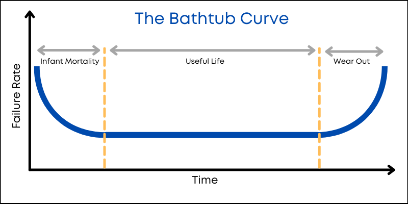
In general, the failure characteristics of many products follow the bathtub curve through their lifecycle. Early failures are addressed by fixing defects. Then, the product remains in operation for a long time with a random, but low and constant failure rate. Lastly, if the product remains in use for a long time period, age will take its toll and the wear out failures are likely to occur.
Reliability Predictions are used to estimate the failure rate of products in the constant failure rate portion, i.e., the useful life phase, of the bathtub curve. Some standards include additional factors to address the early life and wear out portions of the bathtub curve. These factors can be used in addition to the constant failure rate predictions for additional product assessment if desired.
Understanding MTBF, Failure Rate, and Reliability Metrics
As noted, Reliability Prediction standards provide equations to assess the failure rate of electro-mechanical devices. Failure rate (commonly designated as λ) is the number of failures expected over a given time period and is typically expressed in terms of failures/million hours (FPMH) or failures/billion hours (FITs). For example, a failure rate of 10 FPMH indicates that the system is estimated to fail 10 times over one million hours of operation.
Mean Time Between Failure, or MTBF, is equal to the inverse of failure rate (1/λ) when operating in the constant failure rate (useful life) portion of the bathtub curve. MTBF is expressed in terms of hours. In general terms, a system’s MTBF is the average number of hours the given unit will operate before a failure occurs. Analysts may also refer to Mean Time To Failure, or MTTF, as a reliability measure. In general, systems which are repairable tend to use MTBF to evaluate the total time between failures. If a system is not repairable, it means that once a failure occurs the system is down, and MTTF is a more useful metric. Also most applicable to non-repairable systems, MTTFF (Mean Time to First Failure) can also be employed.
These reliability metrics are the output results from Reliability Prediction analyses. In some cases, the term “MTBF Analysis” is used to refer to Reliability Prediction analysis.
Why should I do Reliability Predictions?
One of the first goals in a new product design is to assess reliability. This begins with understanding the factors that drive product performance and identifying potential critical issues that may arise. As a design matures and more detailed information becomes available, targeting possible reliability improvements becomes critical. Reliability Predictions provide information necessary to help achieve your reliability goals in any stage of your product lifecycle.
The central goal of performing Reliability Prediction analysis is to improve product reliability and quality. It is difficult to achieve this goal without measurable statistics. Additionally, it can be especially difficult in the design stage of the product lifecycle to assess reliability metrics before production has started. Reliability Predictions are helpful in this situation by allowing you to complete an MTBF evaluation of your product while design changes that improve reliability and quality can easily be implemented. Reliability Predictions also provide a way to perform What-If? exercises to assess the effect of various design changes on product reliability.

Reliability Predictions can be used starting in early phase design concept and then through to manufacturing and production. In fact, Reliability Predictions are most useful when used throughout your entire product lifecycle and even into next-gen product development. You can start your analysis with as much information as you have to get a quick, early assessment, then refine further as your design matures to get an increasingly more accurate reliability assessment. Then as you move on to future product revisions, you can start with your original analysis and adapt the lessons learned into your next design. In this manner, Reliability Predictions become a key element in your continual improvement process.
What are the benefits of Reliability Predictions?
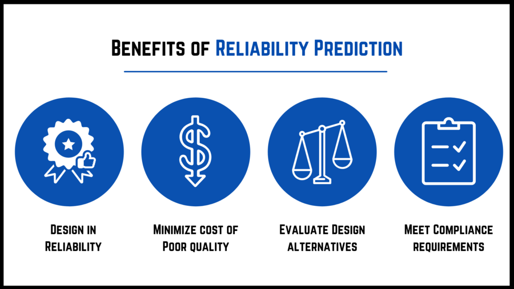
One of the main advantages of Reliability Predictions is that they can be performed during the product design stage, enabling you to preview likely reliability metrics prior to manufacture and deployment. This enables you to design-in reliability, so you can be confident your product will achieve your reliability and quality goals when built.
In the product lifecycle, the cost of correcting a failure dramatically increases along every stage of a product’s life. In early stages, design changes incur minimal cost – only the engineering time associated with the redesign. Design changes required later to correct defects, however, can incur huge costs – manufacturing line downtime, recalls, product replacement, etc. Additionally, there are the immeasurable negative costs to your reputation and corporate standing. Reliability Predictions are a fundamental and proven approach for early reliability assessment that help ensure the cost of design changes is minimized.
Reliability Predictions also provide a way to perform design comparison analyses, which allow you to quantifiably measure the reliability of various design alternatives. For example, you may have two proposed designs for a specific subsystem. Using Reliability Prediction MTBF analysis, you can view the predicted reliability profile of each design and make a decision based on clear metrics.
Lastly, Reliability Predictions may be performed to meet compliance requirements. In some situations, vendors may be contractually obligated to meet specific MTBF goals. Armed with MTBF assessments from Reliability Prediction analyses, your compliance requirements can be attained.
Check out our blog post for more about the benefits of MTBF analysis.
An Example Reliability Prediction Calculation
A Reliability Prediction analysis is a comprehensive evaluation of a system based on all individual components. The system can be as complex as you desire – from a single circuit board to a large multifaceted product such as an airplane or automobile. However, in either case, the underlying fundamentals are similar.
The first step in a Reliability Prediction analysis is to create a list of all the devices that are used in your product. This includes everything from integrated circuits, to resistors, capacitors, and even mechanical components. Often, you may obtain this information from your CAD tool’s product design file, or from a BOM (Bill of Materials) which is a list of components in a system.
It is typically easiest to use a hierarchical structure to break your system down into manageable subassemblies. For example, if you are analyzing a Drone, you may break it down into a structure like this:
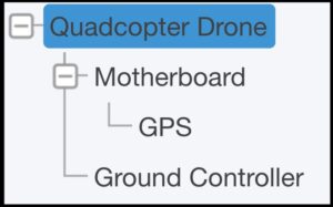
Then, you delineate all the components in each subassembly. For the example above, the Motherboard may include the following list of devices:

As previously explained, you must then select a standard to use for your Reliability Prediction Analysis. For our example, we’ll use the MIL-HDBK-217 F Notice 2 standard. We’ll focus on a single device to explain how the failure rate calculation is completed.
Example Part Calculation
Let’s take a look at the first part identified in our parts list for the Motherboard: a microprocessor. To find the failure rate calculation for this device, we turn to the MIL-HDBK-217 standard and see that Section 5.1 for “Microcircuits, Gates/Logic Arrays and Microprocessors” is applicable.
The equation for Microcircuits, Gate/Logic Arrays and Microprocessors from Section 5.1 is:
λP = (C1 * πT + C2 * πE) * πQ * πL
where λP is the failure rate in failures/million hours (or failures/106 hours, or FPMH).
The variables in the equation represent:
- C1 factors in the complexity of the device, such as the number of gates or transistors
- πT factors in the ambient temperature and any temperature rise associated with the device
- C2 factors in the package of the device, or how it is manufactured and placed in the system, such as surface mounted and/or hermetically sealed
- πE factors in the environment that the device is operating in, such as in space, in an aircraft, in the sea, on the ground, etc.
- πQ factors in the quality of the device based on how it is procured
- πL factors in how long the device has been manufactured
At this point we need to evaluate the contributing variables – the Pi Factors and C Factors – of the equation. Again, we turn to the standard to evaluate.
Evaluate Pi Factors and C Factors
The C1, or die complexity, factor is found using this table from the MIL-HDBK-217 standard:
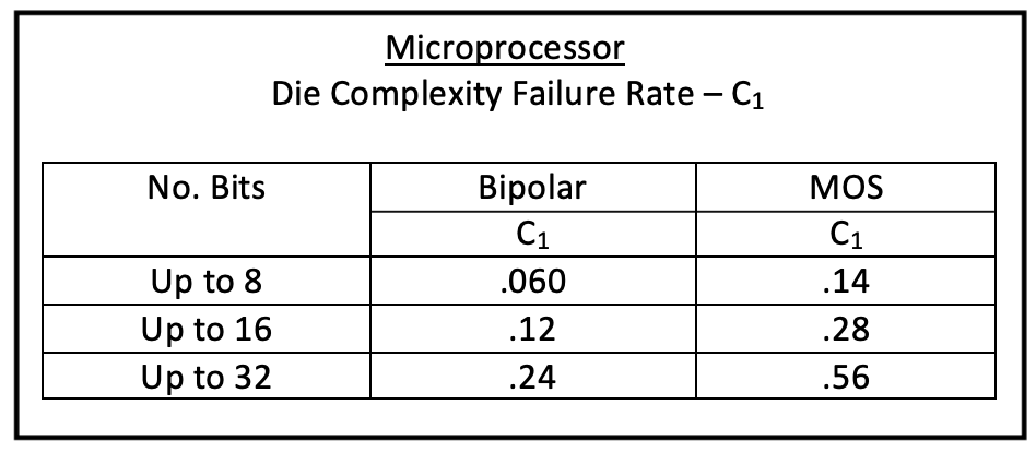
The device in our design is a bipolar 32-bit microprocessor, so the C1 value is 0.24.
The πT, or temperature, factor is calculated based on the given equation:
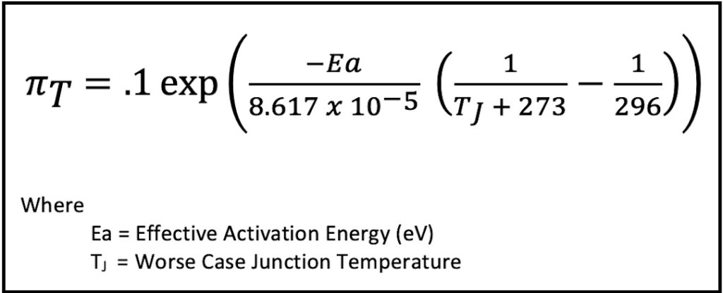
MIL-HDBK-217 provides a table to assess the value of Ea based on the device Technology Type and Junction Temperature. The microprocessor is a LSTTL device with a junction temperature (TJ) of 77 degrees C, so resulting πT is equal to 1.80.
The C2, or package type, factor is computed based on an equation:

Our device is a Nonhermetic DIP package with 128 pins, which results in a C2 factor of 0.068.
πE is determined from the following table:
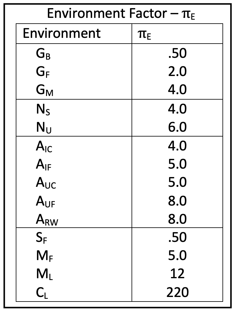
Our operating environment is Aircraft Rotary Winged (ARW), so πE = 8.0.
πL is based on the following table:
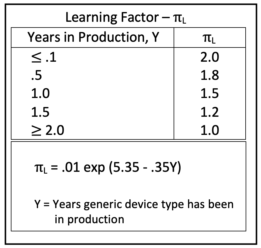
Our device’s years in production is more than 2 years, so πL = 1.0.
Lastly, we obtain πQ from the following table:
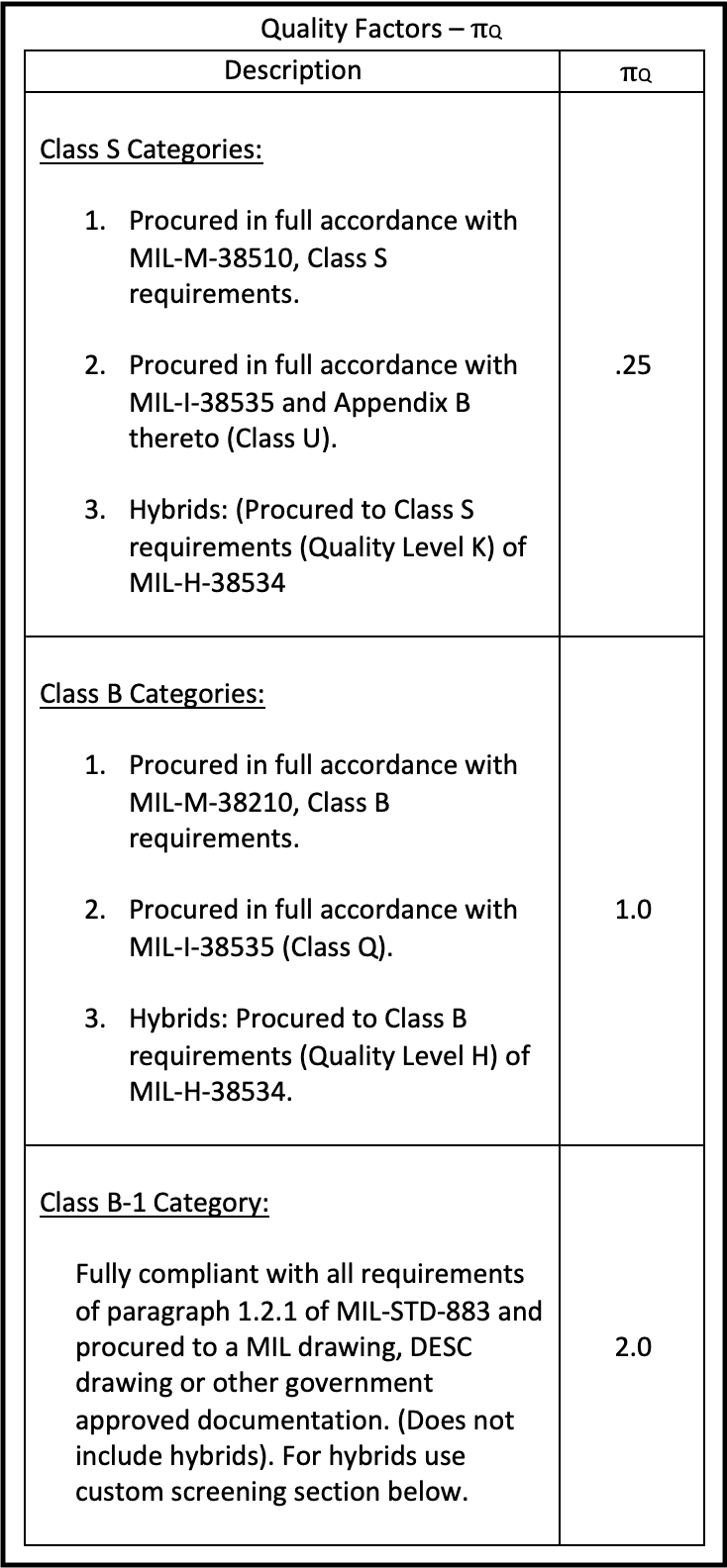
Note: MIL-HDBK-217 includes additional πQ table for custom screened and commercial devices.
Our device quality level is B-1, so πQ = 2.0.
Calculate Failure Rate
Now, we enter these values into our failure rate equation. The resulting failure rate for our microprocessor is:
λP = (C1 * πT + C2 * πE) * πQ * πL
= (0.24 * 1.80 + 0. 068 * 8.0) * 2.0 * 1.0
= 1.95 FPMH (Failure per Million Hours)
With a Failure Rate of about 2 FPMH, we expect that part to fail two times in one million hours.
Complete Reliability Prediction
The same type of process is then required for each component that makes up the subassembly under analysis. This means that, for our example Motherboard the same procedure is needed for each of the other devices, which includes 4 other integrated circuits, a connector, a capacitor, and a USB port. The equations and underlying factors varying depending on the particular device type and can be found in the MIL-HDBK-217 standard.
Once the failure rates of the components are calculated, they are summed to obtain the failure rate of the Motherboard. This process then iterates up the product tree until all failure rates are computed and the overall failure rate of the Quadcopter Drone itself can be determined.
How do I perform a Reliability Prediction?
Using a Reliability Prediction Software Tool
As you can see from the preceding example, performing a Reliability Prediction on a product or system of any size can be time-consuming and error prone if done manually. Even if done with a spreadsheet tool, the process is still tedious and difficult. This is why Reliability Prediction analyses are most often performed using a software tool such as Relyence. Relyence Reliability Prediction supports all the most widely accepted standards for Reliability Prediction analysis. Importantly, it also streamlines the data entry and analysis processes, for efficiency and accuracy.
For example, using the microprocessor example from above, Relyence Reliability Prediction requests the necessary data parameters in an easy-to-read form and presents a list of valid choices where applicable.
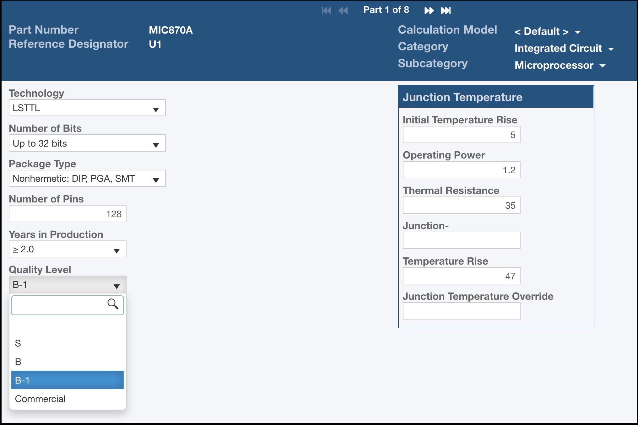
In addition, you do not even need to enter all the exact data parameters if you do not yet know them. Relyence Reliability Prediction has a built-in database of average default values to use when data parameters are not available. This enables you to perform a prediction analysis at any point in your design process, and then continually update data parameter values as your design becomes finalized. If you do not know the appropriate value for a requested parameter, leave the field blank and Relyence Reliability Prediction will use the supplied default value.
To perform a Reliability Prediction on your system using Relyence, you input the components and as much data you know and simply press “Calculate”. The Relyence calculation engine goes through all the necessary computations and provides your system results in seconds.
Where Do I Find the Part Data Needed for Reliability Prediction Analysis?
As demonstrated in the example above, one important element of performing a failure rate calculation is knowing the values of the data parameters needed to solve the equations. For the example microprocessor, the data required includes:
- The technology type
- The number of bits
- The operating temperature
- The package type
- The number of pins
- The operating environment
- The number of years the device has been in production
- The quality level of procurement
The required data parameters vary for each device and across standards. Therefore, there is a great deal of information that must be gathered to complete a Reliability Prediction analysis. How do you obtain this data? The information is found across several sources, most commonly:
- Manufacturer device data sheets
- BOM (Bill of Materials) files
- Design drawings
- Design engineers
In general, non-design specific information such as number of pins, rated stress factors, etc., can be found in device data sheets. Operating, or design specific data, such as temperature, quality, and operating stresses must be obtained from design documents and design engineers.
An important benefit of Reliability Prediction software is that device manufacturer information can be retrieved automatically from built-in part databases. This eliminates the need to spend time gathering all this data. There are often other unique techniques to help in information gathering, such as decoding part descriptions to extract part data, as Relyence’s Intelligent Part MappingTM does.
Additionally with Reliability Prediction software, you can leave unknown data blank and the software package will use average data values to complete Reliability Prediction calculations. This enables you to perform failure rate and MTBF calculations early on and then refine the analysis as your design evolves and data parameters become known.
The Reliability Prediction Process
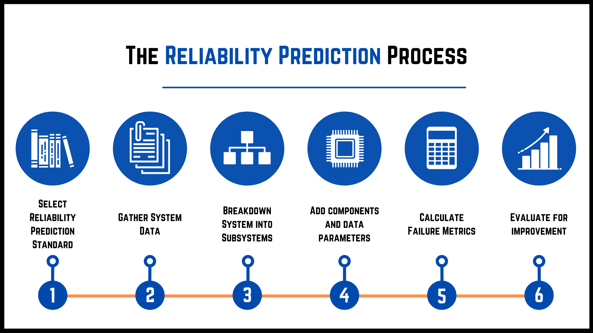
Once you have a Reliability Prediction tool in place, the steps to perform a Reliability Prediction are straightforward:
- Select Reliability Prediction standard: Choose the prediction standard or combination of standards that are most applicable for your requirements.
- Gather system data: Acquire all the necessary information about your product, including all subassemblies in your system and their component parts. Data may be found in design documents, BOM (Bill of Materials), and from design engineers.
- Break the system down into subsystems: Determine how you are going to break down your system into a hierarchical structure for analysis.
- Add components and data parameters: Add all the devices in each subassembly and the associated part data needed for analysis. You may be able to import this information from your BOMs and use databanks for data parameter retrieval.
- Calculate failure metrics: Compute failure rate and MTBF values for the system and all subassemblies.
- Evaluate for improvement: Review the results and make a plan for improvement if necessary.
For an in-depth explanation of the Reliability Prediction process, see our MTBF Analysis in Six Steps article which provides a detailed guide of the steps outlined here.
Conclusion
The best-in-class Relyence Reliability Prediction supports complete and accurate analyses based on all the widely accepted standards: MIL-HDBK-217, Telcordia, 217Plus, IEC 61709, SN 29500, NSWC Mechanical, ANSI/VITA 51.1, and China’s 299C. It offers a host of features to make your reliability prediction tasks quick and efficient, including all those outlined in this article. Relyence Reliability Prediction provides a solid foundation for all your analysis needs and fills an essential role in your reliability and quality analysis tool set.
Contact us today so we can talk about your Reliability Prediction needs and how Relyence Reliability Prediction can help, or sign up today for our free trial to see Relyence Reliability Prediction in action.


