What is MTBF?
MTBF analysis is used to assess the MTBF, or Mean Time Between Failures, of a system or product. MTBF is a useful unit of measure for evaluating failure characteristics. It is the average amount of time a repairable system can be expected to operate between failures. It is commonly expressed in terms of hours. For example, an MTBF of 1000 hours indicates that a system, on average, will successfully operate for 1000 hours before experiencing a failure. However, this is just a predicted or estimated value, it does not indicate that the system will fail precisely at 1000 hours!
MTBF can be computed using the failure rate of a system in its useful life period, or the part of the product lifecycle where the failure rate of the system is constant. The useful life section is the central and longest portion of the product lifecycle as described by the bathtub curve. In this timeframe, there is a relationship between MTBF and failure rate: MTBF is the inverse of failure rate. In other words, if the failure rate is known, then MTBF is equal to 1 / failure rate. So, if I know the failure rate of my system is 500 FPMH (failures per million hours), then the MTBF of my system is equal to 1 / 500 failures / 1,000,000 hours, or 2000 hours.
How is MTBF Calculated?
Due to the relationship between failure rate and MTBF, techniques that compute failure rates can be used for MTBF analysis. Failure rates of electromechanical systems can be computed using analytical techniques and methodologies well-known and established in the reliability engineering field. The most well-known and widely used approach for failure rate analysis is Reliability Prediction. This is why Reliability Prediction analysis is a valuable method for performing MTBF analysis.
Reliability Predictions are often used in product design and development as part of reliability and quality continuous improvement efforts. Reliability Predictions are used to predict the failure profiles of devices in the constant failure rate portion of the product lifecycle. The results of Reliability Prediction analyses are failure rate, MTBF, and other related reliability metrics.
Reliability Prediction analysis is almost exclusively performed using a software package expressly designed for that purpose. Because MTBF analysis using Reliability Prediction is a detailed, mathematical-based methodology, software tools are key to efficient analyses. Reliability Prediction software is the most effective way to calculate failure rate and MTBF.
Other reliability engineering tools also provide valuable ways to assess MTBF. For example, Weibull analysis predicts failure trends based on life data and ALT (Accelerated Life Testing) analysis predicts failure trends based on test data. Notably, Reliability Block Diagram (RBD) uses high-powered mathematical techniques to model complex systems using block diagrams. Most commonly, the term MTBF analysis is used in reference to the analysis performed using Reliability Prediction standards, which will be the focus of this article.
What are the Steps for Performing MTBF Analysis?
When using Reliability Prediction software tools for MTBF analyses, there is a straightforward, step-by-step process to follow. This step-by-step process can also be done iteratively, so that as the product under analysis evolves and changes, the same steps can be repeated to refine the MTBF results.
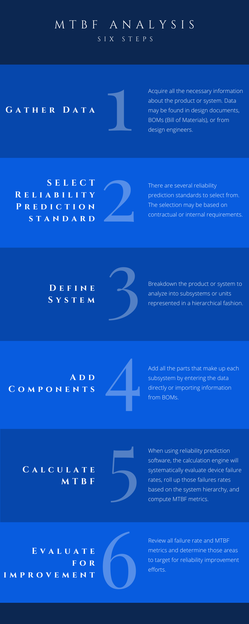
The six-step process for MTBF analysis is:
- Gather your data
- Select which Reliability Prediction standard to use
- Define your system
- Add components
- Calculate MTBF
- Evaluate for improvement
Step 1. Gather Your Data
To evaluate your system MTBF using Reliability Prediction techniques, the first step is to acquire all the necessary information about your product or system. You will need to know the following:
- The overall structure or design of the system or product you are analyzing
- The components that are included in each subsystem or unit of your product
- The operating conditions for your product, such as the environment and temperature
- The operating stresses of the components, such as operating voltages and currents
- If available, lab test data and/or field data (such as accumulated in CAPA or FRACAS)
Much of this data can be obtained from product design drawings, BOMs (Bill of Materials), or from design engineers.
It is important to note that detailed data such as operating stresses of all the system components is not required in order to begin MTBF analysis. When using Reliability Prediction software, accepted default values are used for unknown data parameters. The minimum you need to start your MTBF analysis is a listing of components, which is commonly available from BOMs.
As data parameters become finalized during the design stage, the Reliability Prediction analysis can be updated. As more and more data is acquired, the failure rate assessments will become more accurate.
Lab testing data or data from product use in the field can be used to further refine your MTBF analysis. This data is used in conjunction with the design data to adjust the predicted values based on this real-world information.
Step 2. Select which Reliability Prediction Standard to Use
Deciding which Reliability Prediction standard to employ for analysis may not always be required. For example, contractual requirements may designate the standard to be used. In other cases, your organization may have internal requirements that dictate the standard to employ. In these situations, you must comply with the requirements and no decision is needed.
However, if you do not have a requirement explicitly designated, you have a choice of standards to select from. There is no right or wrong decision, you just need to make a judgement call based on the standard that best meets your particular needs. It also should be noted that you can use multiple standards for an analysis. See our informative guide for details on the available standards, how to use a combination of standards, and advice on how to choose.
There are several widely accepted Reliability Prediction standards:
- MIL-HDBK-217
- Telcordia
- 217Plus
- IEC 61709
- SN 29500
- NSWC Mechanical
- ANSI/VITA 51.1
- China’s GJB/z 299
In addition, the NPRD/EPRD databases are often used in conjunction with standards when performing reliability prediction analyses. These databases are not standards-based, but provide failure rates for devices, components, and subsystems based on real world accumulated data.
Failure Rate Equations
Each Reliability Prediction standard offers a set of mathematical formulas which are used to calculate the failure rate of a variety of electromechanical components. These equations were built by analyzing a huge amount of field data over a long period of time. Statistical analysis was then performed to develop the equations which best modeled the failure characteristics of the accumulated data.
For example, an equation from MIL-HDBK-217 for Integrated Circuits (ICs) is:
λp = (C1 * πT + C2 * πE) * πQ * πL
where:
λp is the failure rate in failures/million hours (or failures/10e6 hours, or FPMH)
and:
- C1 factors in the complexity of the device, such as the number of gates or transistors
- πT factors in the ambient temperature and any temperature rise associated with the device
- C2 factors in the package of the device, or how it is manufactured and placed in the system, such as surface mounted and/or hermetically sealed
- πE factors in the environment that the device is operating in, such as in space, in an aircraft, in the sea, on the ground, etc.
- πQ factors in the quality of the device based on how it is procured
- πL factors in how long the device has been manufactured
As you can see, the equations are quite detailed. Plus, they are specific to each Reliability Prediction standard and each type of device. So, for instance, the equation for resistors is different than the example equation shown above for ICs. The specific Pi factors (π) and the data they are dependent on vary across device types. You can see why employing Reliability Prediction software is essential to performing efficient MTBF analysis!
The failure rate of each component in your system is analyzed using these equations, and then the sum total of all the component failure rates is the overall failure rate of the system.

MIL-HDBK-217
MIL-HDBK-217, or Military Handbook: Reliability Prediction of Electronic Equipment, is one of the most widely used and accepted Reliability Prediction standards. It was one of the first models developed, and most other reliability standards available today have their roots in MIL-HDBK-217. Initially designed for use in defense and military applications, MIL-HDBK-217 is now widely used in all industry sectors. The latest version is MIL-HDBK-217F Notice 2.
Telcordia
Telcordia, or Telcordia: Reliability Prediction Procedure for Electronic Equipment, Special Report SR-332, is also a broadly used standard. Historically, Telcordia was often called the Bellcore standard. Initially, the Bellcore/Telcordia standard was developed for use in the telecommunications industry. Today, Telcordia is used and accepted across the spectrum of industry sectors. Telcordia Issue 4 is the latest Telcordia Reliability Prediction standard.
217Plus
217Plus™, or Handbook of 217Plus Reliability Prediction Models, was developed by Quanterion Solutions. Work on 217Plus was started under Department of Defense contracts with the Reliability Analysis Center (RAC) and Reliability Information Analysis Center (RIAC) and was released originally under the name PRISM. The failure rate models of 217Plus have their roots in MIL-HDBK-217 but have enhancements to include the effects of operating profiles, cycling factors, and process grades on reliability. The most recent version is 217Plus 2015 Notice 1.
IEC 61709
IEC 61709, developed by the International Electrotechnical Commission (IEC), is entitled “Electric components – Reliability – Reference conditions for failure rates and stress models for conversion.” It provides a method to convert failure rates from reference conditions to different operating conditions for a variety of electromechanical components. Therefore, the models in the IEC 61709 standard require a “base” or “reference” failure rate to be defined in order to perform analysis. IEC 61709 provides stress models to compute component failure rates by adjusting the reference failure rates to account for different operating conditions.
SN 29500
Originally from Siemens, SN 29500 covers a broad range of devices including resistors, capacitors, integrated circuits, and connectors. It takes into account the effects of operating temperature, applied stress, and environmental conditions when computing failure metrics. Primarily used in Europe by businesses serving the industrial automation, power generation, transportation, and commercial electronics sectors, SN 29500 is often the preferred or required method for reliability predictions.
ANSI/VITA 51.1
ANSI/VITA 51.1, or American National Standards Institute VITA 51: Reliability Prediction MIL-HDBK-217 Subsidiary Specification, is a collaborative industry standard that provides recommended modifications to the MIL-HDBK-217F Notice 2. As noted in ANSI/VITA 51.1, it is not a revision of MIL-HDBK-217, but a “standardization of the inputs to the MIL-HBDK-217F Notice 2 calculation to give more consistent MTBF numbers.” If you choose to use ANSI/VITA 51.1, it must be used in conjunction with MIL-HDBK-217.
China’s GJB/z 299
China’s GJB/z 299, or GJB/Z 299: Reliability Prediction Model for Electronic Equipment, is mostly used in the Chinese market. It also has its roots in MIL-HDBK-217. It may be useful for companies doing business with Chinese manufacturers or utilizing Chinese made components. The most recent version is China’s GJB/z 299C.
NPRD/EPRD Databases
The NPRD (Non-electronic Parts Reliability Data) and EPRD (Electronic Parts Reliability Data) are not standards based on failure rate equations, but rather they are databanks that include failure data on a wide range of electrical components and electromechanical parts and assemblies based on real-world usage. NPRD and EPRD are helpful because they can provide failure rate estimates for devices not modeled with equations. Or you may prefer to use actual field-based metrics rather than the equation-based predictive models. The latest versions of these databases, NPRD-2016 and EPRD-2014, can be used alongside the prediction standards and work well together.
3. Define your System
Step 3 is where your MTBF analysis begins in earnest. At this point you have completed the groundwork to begin evaluation: you have the necessary data and have selected a standard to use.
Start by reviewing the overall structure of your product or system. At this step is it important to decide the breadth of your analysis. For example, perhaps your organization is responsible for only a single subsystem of a larger system. In this situation, you may decide to concentrate your analysis only on the part of the system you are working on. Or perhaps you are still interested in the overall MTBF, so you still want to include the entire system in your analysis. Your analysis can be set up to handle either of these two ends of the spectrum, or any configuration between.
Begin by defining the hierarchical representation of what you intend to analyze. By defining your system in a hierarchical manner, you can easily see the contributions of the separate subsystems to the overall failure rate. This encapsulation has several benefits. First, it enables you to better organize your tasks by allowing you to concentrate on one subsystem at a time. Secondly, it allows you to more easily employ a team approach to divide up the work among team members. Lastly, as you move into the task of improvement, you will easily be able to determine where you should most effectively spend your effort.
For example, if analyzing a drone, we could breakdown the drone into subsystems of drone body and ground controller. We can then further breakdown the drone body into motherboard, GPS, and camera.
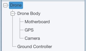
Example system breakdown for analyzing a drone
4. Add Components
Once your subsystems are defined, you add all the parts that make up each subsystem. For example, if you are looking at a circuit board, you add in each and every component on that circuit board. This list includes all devices such as resistors, capacitors, ICs, etc.
Oftentimes, this information is available in your BOM. In many cases, you can directly import this data into your Reliability Prediction software. This makes the entry of this data much quicker and easier. You simply import your BOM file and the information is immediately available in your analysis.
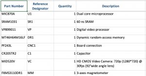
Example BOM which can be imported into Relyence Reliability Prediction software
As noted above, for each part type, there are a number of specific data parameters that are used to compute the device failure rate. Once the components are in your analysis, enter as much of the specific data that you currently have available.
Reliability Prediction software tools have many features that make this part of the process easier. For example, Relyence Reliability Prediction includes several notable features that streamline this process:
- For any unknown data parameters, reasonable default values are used.
- An extensive built-in component library is automatically activated to retrieve known data parameters, such as rated voltages, number of pins, etc.
- A unique Intelligent Part MappingTM feature enables part descriptions to be decoded to retrieve as much information as possible.
- You can create and continually update your own library of components for easy retrieval and reuse.
- You can easily search all libraries, including the NPRD and EPRD databases, to look up and retrieve device data.
- The Knowledge Bank capability enables you to store and reuse entire subsystems.
5. Calculate MTBF
Now that all your data is entered, the central event of your analysis can be performed! When using Reliability Prediction software, this is nothing more than clicking a button. Once the calculation engine is engaged, the software will systematically evaluate all device failure rates, roll up those failures appropriately based on your system hierarchy, and produce the vital MTBF metrics.
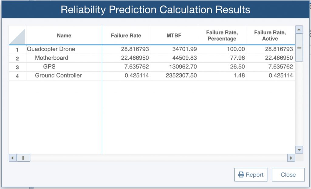
Example results of Reliability Prediction analysis
Using Reliability Prediction software, you can generate a wide range of reports for inclusion in presentations or for compliance requirements.
As your design progresses, design changes occur, and as more data becomes available, you can update your Reliability Prediction analysis with the newly acquired information. You can then recalculate your failure rate and MTBF metrics in order to continually keep track of changes to your system reliability.
6. Evaluate for Improvement
Once calculations are complete, you review the results. You may need to work to improve the MTBF of your system. For example, you may have contractual requirements to meet a specific MTBF goal. Or you may have internal requirements for quality objectives that must be met.
By looking at individual parts and their associated π factors (or pi factors), you can determine how effective particular design changes will be. For example, if the πT factor for a particular device is very high, that means that lowering the device temperature (the determining factor for πT) will decrease the failure rate. Perhaps adding a fan to this component can lower its operating temperature, resulting in an improved MTBF.
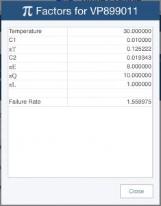
Example Pi factor calculation
Performing trade studies, or what-if? analyses, are a useful way to consider various design options to improve overall system reliability. What-if? analyses enable you to change data parameters and quickly assess the resulting effect on failure metrics. Using the same example noted above, what-if? analysis allows you to change device temperatures, rerun calculations, and view the results of this change.
Dashboards are also very valuable for an overview of system reliability metrics. For example, you can view a chart that includes the components with the highest overall failure rates, or a pie chart to easily view the contributions each subsystem has to the overall system failure rate. This type of information enables you to quickly zero in on areas where improvements can have the greatest impact.
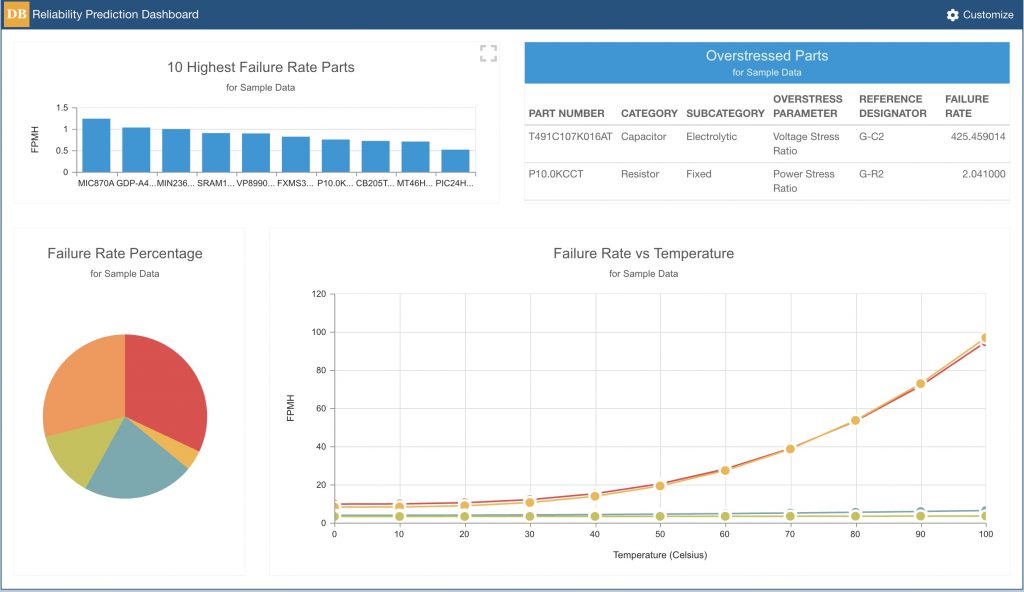
Example Relyence Reliability Prediction Dashboard
Relyence Reliability Prediction Software
Relyence Reliability Prediction provides an efficient platform for performing MTBF analysis based on Reliability Prediction standards. Beyond the support for all the standards, Relyence Reliability Prediction includes a long list of capabilities and features that allow you to perform analyses with unparalleled efficiency. Some notable additions include component libraries, What-If? trade studies, Intelligent Part MappingTM, derating analysis, dashboards, allocation analysis, mission profile calculations, and more.
If you are interested in learning more about Relyence Reliability Prediction or our integrated Relyence Studio platform sign up today for your own no-hassle free trial. Or, feel free to contact us to discuss your needs or schedule a personal demo.


